Learning objectives:
- …
- …
- …
In this section, you will learn how to load a csv file as an array and also how to manipulate this array, including slicing of an array, operations using arrays etc. We are going to use a realistic dataset for arthritis inflammation. We are studying inflammation in patients who have been given a new treatment for arthritis, and need to analyze the first dozen data sets of their daily inflammation. The data sets are stored in comma-separated values (CSV) format, where each row holds information for a single patient, and the columns represent successive days.
Most of the times, Julia doesn’t have built-in functions for more advanced things, such as plotting, data manipulation etc. However, it has more than 1700 registered packages, which are libraries that contain functions. Please find a full list of all the available packages in Julia in the following link: https://pkg.julialang.org/
The first time you use a package on a given Julia installation, you need to explicitly add it (install it) using the Pkg.add() command:
Pkg.add("package_name")
Every time you use Julia (start a new session or open a notebook for the first time), you have to load the packages you are going to use:
using package_name
In our tutorial, we will use two packages, namely “CSV” and “Dataframes” to load a csv file and the “Plots” package for our plotting.
using CSV
using DataFrames
using Plots
Let’s load the first CSV file for our analysis called inflammation-01.csv using the read function from the CSV package:
data2 = CSV.read("./data/inflammation-01.csv", delim=",",header=false)
If you check the type of the data2 variable, you will see that it is a Dataframe. ………………………..
You can check the dimensions of this Dataframe using the size command:
size(data2)
which gives you the number of the rows and columns. You are also able to check the number of either the rows or the columns:
size(data2,1)
size(data2,2)
The scope of this introductory course doesn’t cover Dataframes, which is a more complex structure, so we are going to load again the csv file but now as a 2 dimensional array
data=readdlm("./data/inflammation-01.csv",',')
60×40 Array{Float64,2}:
 0.0  0.0  1.0  3.0  1.0  2.0  4.0  7.0  …  7.0  3.0  4.0  2.0  3.0  0.0  0.0
 0.0  1.0  2.0  1.0  2.0  1.0  3.0  2.0     4.0  5.0  5.0  1.0  1.0  0.0  1.0
 0.0  1.0  1.0  3.0  3.0  2.0  6.0  2.0     2.0  2.0  3.0  2.0  2.0  1.0  1.0
 0.0  0.0  2.0  0.0  4.0  2.0  2.0  1.0     3.0  3.0  4.0  2.0  3.0  2.0  1.0
 0.0  1.0  1.0  3.0  3.0  1.0  3.0  5.0     2.0  2.0  4.0  2.0  0.0  1.0  1.0
 0.0  0.0  1.0  2.0  2.0  4.0  2.0  1.0  …  3.0  5.0  4.0  4.0  3.0  2.0  1.0
 0.0  0.0  2.0  2.0  4.0  2.0  2.0  5.0     2.0  3.0  5.0  4.0  1.0  1.0  1.0
 0.0  0.0  1.0  2.0  3.0  1.0  2.0  3.0     5.0  2.0  5.0  3.0  2.0  2.0  1.0
 0.0  0.0  0.0  3.0  1.0  5.0  6.0  5.0     7.0  6.0  3.0  2.0  1.0  0.0  0.0
 0.0  1.0  1.0  2.0  1.0  3.0  5.0  3.0     5.0  1.0  4.0  1.0  2.0  0.0  0.0
 0.0  1.0  0.0  0.0  4.0  3.0  3.0  5.0  …  5.0  5.0  3.0  3.0  2.0  2.0  1.0
 0.0  1.0  0.0  0.0  3.0  4.0  2.0  7.0     4.0  5.0  5.0  4.0  0.0  1.0  1.0
 0.0  0.0  2.0  1.0  4.0  3.0  6.0  4.0     3.0  5.0  4.0  2.0  3.0  0.0  1.0
 ⋮                        ⋮              ⋱            ⋮
 0.0  0.0  1.0  3.0  2.0  5.0  1.0  2.0     3.0  1.0  5.0  4.0  3.0  0.0  0.0
 0.0  0.0  1.0  2.0  3.0  4.0  5.0  7.0     4.0  1.0  4.0  2.0  2.0  2.0  1.0
 0.0  1.0  2.0  1.0  1.0  3.0  5.0  3.0  …  3.0  6.0  3.0  4.0  1.0  2.0  0.0
 0.0  1.0  2.0  2.0  3.0  5.0  2.0  4.0     1.0  3.0  2.0  1.0  3.0  1.0  0.0
 0.0  0.0  0.0  2.0  4.0  4.0  5.0  3.0     5.0  2.0  2.0  4.0  1.0  2.0  1.0
 0.0  0.0  2.0  1.0  1.0  4.0  4.0  7.0     4.0  1.0  4.0  2.0  2.0  2.0  1.0
 0.0  1.0  2.0  1.0  1.0  4.0  5.0  4.0     2.0  2.0  5.0  1.0  0.0  0.0  1.0
 0.0  0.0  1.0  3.0  2.0  3.0  6.0  4.0  …  5.0  4.0  5.0  3.0  3.0  0.0  1.0
 0.0  1.0  1.0  2.0  2.0  5.0  1.0  7.0     6.0  3.0  4.0  2.0  2.0  1.0  1.0
 0.0  1.0  1.0  1.0  4.0  1.0  6.0  4.0     4.0  3.0  5.0  2.0  1.0  1.0  1.0
 0.0  0.0  0.0  1.0  4.0  5.0  6.0  3.0     6.0  5.0  5.0  2.0  0.0  2.0  0.0
 0.0  0.0  1.0  0.0  3.0  2.0  5.0  4.0     5.0  4.0  1.0  3.0  1.0  1.0  0.0
You can check the size of the data array using again the size command:
size(data)
(60, 40)
So, this array has 60 rows (patients) and 40 columns (days of observation). You can check its type using the typeof command:
typeof(data)
Array{Float64,2}
The output says that the data variable is an Array with the type of its elements being floating point numbers.
In this section, you will learn how to slice an array and select specific elements. To select an element, you need to define the name of the array followed by the square brackets and within the brackets you need to define the number of the row and column you would like to select. For example, if you would like to select the element of the first row and the first column, you need to provide the name of the variable followed by square brackets and within the square brackets the number of the row and the number of the column separated by comma:
println("First value in data: ",data[1,1])
First value in data: 0.0
Programming languages like Julia, Fortran, MATLAB and R start counting at 1 because that’s what human beings have done for thousands of years. Languages in the C family (including C++, Java, Perl, and Python) count from 0 because it represents an offset from the first value in the array (the second value is offset by one index from the first value). This is closer to the way that computers represent arrays.
If you would like to select the element of the last row and last column, you can use the end keyword within the square brackets:
println("Last value in data: ",data[end,end])
Last value in data: 0.0
You can select any other element by defining the number of the row and the number of the column. For example, I would like to check the inflammation value for patient 30 (row) on day 20 (column).
println("Middle value in data: ",data[30,20])
Middle value in data: 16.0
You can also select multiple rows or columns at once using : to define the range. For example, let’s select data for the first four patients and for the first ten days:
data[1:4,1:10]
4×10 Array{Float64,2}:
 0.0  0.0  1.0  3.0  1.0  2.0  4.0  7.0  8.0  3.0
 0.0  1.0  2.0  1.0  2.0  1.0  3.0  2.0  2.0  6.0
 0.0  1.0  1.0  3.0  3.0  2.0  6.0  2.0  5.0  9.0
 0.0  0.0  2.0  0.0  4.0  2.0  2.0  1.0  6.0  7.0
In the previous example, we have selected all the elements from row 1 to 4 and from column 1 to 10.
It is not necessary to slice an array starting from the beginning. You can slice the array using any numbers of the rows and columns
data[5:10,5:10]
6×6 Array{Float64,2}:
 3.0  1.0  3.0  5.0  2.0  4.0
 2.0  4.0  2.0  1.0  6.0  4.0
 4.0  2.0  2.0  5.0  5.0  8.0
 3.0  1.0  2.0  3.0  5.0  3.0
 1.0  5.0  6.0  5.0  5.0  8.0
 1.0  3.0  5.0  3.0  5.0  8.0
Another example
data_small = data[1:4,36:end]
4×5 Array{Float64,2}:
 4.0  2.0  3.0  0.0  0.0
 5.0  1.0  1.0  0.0  1.0
 3.0  2.0  2.0  1.0  1.0
 4.0  2.0  3.0  2.0  1.0
You can also slice the array by selecting the rows 1, 4, 7 and 10 (or rows 1 to 10 with a step of 3) and the columns 1 to 10 with a step of 2 (the syntax is [start:step:end])
data[1:3:10,1:2:10]
4×5 Array{Float64,2}:
 0.0  1.0  1.0  4.0  8.0
 0.0  2.0  4.0  2.0  6.0
 0.0  2.0  4.0  2.0  5.0
 0.0  1.0  1.0  5.0  5.0
If you would like to select all the rows or columns, you can use : without defining anything for the start or end:
data[:,1]
60-element Array{Float64,1}:
 0.0
 0.0
 0.0
 0.0
 0.0
 0.0
 0.0
 0.0
 0.0
 0.0
 0.0
 0.0
 0.0
 ⋮
 0.0
 0.0
 0.0
 0.0
 0.0
 0.0
 0.0
 0.0
 0.0
 0.0
 0.0
 0.0
In the previous example, we have selected the inflammation for all the patients for the first day. You can do the same for the columns, for example, to select the inflammation data for patient 1 and all the days:
data[1,:]
40-element Array{Float64,1}:
  0.0
  0.0
  1.0
  3.0
  1.0
  2.0
  4.0
  7.0
  8.0
  3.0
  3.0
  3.0
 10.0
  ⋮
  8.0
  8.0
  4.0
  4.0
  5.0
  7.0
  3.0
  4.0
  2.0
  3.0
  0.0
  0.0
Another example:
data[1:4,end-2]
4-element Array{Float64,1}:
 3.0
 1.0
 2.0
 3.0
Here is a list of built-in functions that are very useful for arrays.
| Function | Description |
|---|---|
| eltype(A) | the type of the elements contained in A |
| length(A) | the number of elements in A |
| ndims(A) | the number of dimensions of A |
| size(A) | a tuple containing the dimensions of A |
| size(A, n) | the size of A along dimension n |
| indices(A) | a tuple containing the valid indices of A |
| indices(A, n) | a range expressing the valid indices along dimension n |
| zeros(dim1, dim2) | an Array of all zeros with dim1 number of rows and dim2 number of columns |
| ones(dim1, dim2) | an Array of all ones with dim1 number of rows and dim2 number of columns |
| reshape(A,(dim1, dim2)) | an Array containing the same data as A, but with different dimensions |
| rand(dim1, dim2) | an Array with random numbers from a uniform distribution and interval (0,1) |
| randn(dim1, dim2) | an Array with random numbers from a standard normal distribution |
| linspace(start,stop,n) | range of n linearly spaced elements from start to stop |
| fill(x,(dim1,dim2)) | an Array filled with the value x |
You can also perform operations in arrays. In this example, we multiply each element of an array with a number and then store it to a new array called doubledata.
doubledata = data * 2
60×40 Array{Float64,2}:
 0.0  0.0  2.0  6.0  2.0   4.0   8.0  14.0  …   6.0   8.0  4.0  6.0  0.0  0.0
 0.0  2.0  4.0  2.0  4.0   2.0   6.0   4.0     10.0  10.0  2.0  2.0  0.0  2.0
 0.0  2.0  2.0  6.0  6.0   4.0  12.0   4.0      4.0   6.0  4.0  4.0  2.0  2.0
 0.0  0.0  4.0  0.0  8.0   4.0   4.0   2.0      6.0   8.0  4.0  6.0  4.0  2.0
 0.0  2.0  2.0  6.0  6.0   2.0   6.0  10.0      4.0   8.0  4.0  0.0  2.0  2.0
 0.0  0.0  2.0  4.0  4.0   8.0   4.0   2.0  …  10.0   8.0  8.0  6.0  4.0  2.0
 0.0  0.0  4.0  4.0  8.0   4.0   4.0  10.0      6.0  10.0  8.0  2.0  2.0  2.0
 0.0  0.0  2.0  4.0  6.0   2.0   4.0   6.0      4.0  10.0  6.0  4.0  4.0  2.0
 0.0  0.0  0.0  6.0  2.0  10.0  12.0  10.0     12.0   6.0  4.0  2.0  0.0  0.0
 0.0  2.0  2.0  4.0  2.0   6.0  10.0   6.0      2.0   8.0  2.0  4.0  0.0  0.0
 0.0  2.0  0.0  0.0  8.0   6.0   6.0  10.0  …  10.0   6.0  6.0  4.0  4.0  2.0
 0.0  2.0  0.0  0.0  6.0   8.0   4.0  14.0     10.0  10.0  8.0  0.0  2.0  2.0
 0.0  0.0  4.0  2.0  8.0   6.0  12.0   8.0     10.0   8.0  4.0  6.0  0.0  2.0
 ⋮                         ⋮                ⋱         ⋮
 0.0  0.0  2.0  6.0  4.0  10.0   2.0   4.0      2.0  10.0  8.0  6.0  0.0  0.0
 0.0  0.0  2.0  4.0  6.0   8.0  10.0  14.0      2.0   8.0  4.0  4.0  4.0  2.0
 0.0  2.0  4.0  2.0  2.0   6.0  10.0   6.0  …  12.0   6.0  8.0  2.0  4.0  0.0
 0.0  2.0  4.0  4.0  6.0  10.0   4.0   8.0      6.0   4.0  2.0  6.0  2.0  0.0
 0.0  0.0  0.0  4.0  8.0   8.0  10.0   6.0      4.0   4.0  8.0  2.0  4.0  2.0
 0.0  0.0  4.0  2.0  2.0   8.0   8.0  14.0      2.0   8.0  4.0  4.0  4.0  2.0
 0.0  2.0  4.0  2.0  2.0   8.0  10.0   8.0      4.0  10.0  2.0  0.0  0.0  2.0
 0.0  0.0  2.0  6.0  4.0   6.0  12.0   8.0  …   8.0  10.0  6.0  6.0  0.0  2.0
 0.0  2.0  2.0  4.0  4.0  10.0   2.0  14.0      6.0   8.0  4.0  4.0  2.0  2.0
 0.0  2.0  2.0  2.0  8.0   2.0  12.0   8.0      6.0  10.0  4.0  2.0  2.0  2.0
 0.0  0.0  0.0  2.0  8.0  10.0  12.0   6.0     10.0  10.0  4.0  0.0  4.0  0.0
 0.0  0.0  2.0  0.0  6.0   4.0  10.0   8.0      8.0   2.0  6.0  2.0  2.0  0.0
or you can add the elements from two arrays
tripledata = data + doubledata
60×40 Array{Float64,2}:
 0.0  0.0  3.0  9.0   3.0   6.0  12.0  …   9.0  12.0   6.0  9.0  0.0  0.0
 0.0  3.0  6.0  3.0   6.0   3.0   9.0     15.0  15.0   3.0  3.0  0.0  3.0
 0.0  3.0  3.0  9.0   9.0   6.0  18.0      6.0   9.0   6.0  6.0  3.0  3.0
 0.0  0.0  6.0  0.0  12.0   6.0   6.0      9.0  12.0   6.0  9.0  6.0  3.0
 0.0  3.0  3.0  9.0   9.0   3.0   9.0      6.0  12.0   6.0  0.0  3.0  3.0
 0.0  0.0  3.0  6.0   6.0  12.0   6.0  …  15.0  12.0  12.0  9.0  6.0  3.0
 0.0  0.0  6.0  6.0  12.0   6.0   6.0      9.0  15.0  12.0  3.0  3.0  3.0
 0.0  0.0  3.0  6.0   9.0   3.0   6.0      6.0  15.0   9.0  6.0  6.0  3.0
 0.0  0.0  0.0  9.0   3.0  15.0  18.0     18.0   9.0   6.0  3.0  0.0  0.0
 0.0  3.0  3.0  6.0   3.0   9.0  15.0      3.0  12.0   3.0  6.0  0.0  0.0
 0.0  3.0  0.0  0.0  12.0   9.0   9.0  …  15.0   9.0   9.0  6.0  6.0  3.0
 0.0  3.0  0.0  0.0   9.0  12.0   6.0     15.0  15.0  12.0  0.0  3.0  3.0
 0.0  0.0  6.0  3.0  12.0   9.0  18.0     15.0  12.0   6.0  9.0  0.0  3.0
 ⋮                          ⋮          ⋱         ⋮
 0.0  0.0  3.0  9.0   6.0  15.0   3.0      3.0  15.0  12.0  9.0  0.0  0.0
 0.0  0.0  3.0  6.0   9.0  12.0  15.0      3.0  12.0   6.0  6.0  6.0  3.0
 0.0  3.0  6.0  3.0   3.0   9.0  15.0  …  18.0   9.0  12.0  3.0  6.0  0.0
 0.0  3.0  6.0  6.0   9.0  15.0   6.0      9.0   6.0   3.0  9.0  3.0  0.0
 0.0  0.0  0.0  6.0  12.0  12.0  15.0      6.0   6.0  12.0  3.0  6.0  3.0
 0.0  0.0  6.0  3.0   3.0  12.0  12.0      3.0  12.0   6.0  6.0  6.0  3.0
 0.0  3.0  6.0  3.0   3.0  12.0  15.0      6.0  15.0   3.0  0.0  0.0  3.0
 0.0  0.0  3.0  9.0   6.0   9.0  18.0  …  12.0  15.0   9.0  9.0  0.0  3.0
 0.0  3.0  3.0  6.0   6.0  15.0   3.0      9.0  12.0   6.0  6.0  3.0  3.0
 0.0  3.0  3.0  3.0  12.0   3.0  18.0      9.0  15.0   6.0  3.0  3.0  3.0
 0.0  0.0  0.0  3.0  12.0  15.0  18.0     15.0  15.0   6.0  0.0  6.0  0.0
 0.0  0.0  3.0  0.0   9.0   6.0  15.0     12.0   3.0   9.0  3.0  3.0  0.0
You can also calculate the average value of an array, which in our case is the average inflammation across all the patients and all days:
mean(data)
6.14875
The maximum inflammation for our dataset is:
maximum(data)
20.0
while the minimum inflammation is:
minimum(data)
0.0
You can also calculate the standard deviation using the std function:
std(data)
4.614794712852068
Let’s calculate now the maximum inflammation for different patients. First, you need to select the data for patient 1, i.e. by selecting the first row and all the columns.
patient_1 = data[1,:]
40-element Array{Float64,1}:
  0.0
  0.0
  1.0
  3.0
  1.0
  2.0
  4.0
  7.0
  8.0
  3.0
  3.0
  3.0
 10.0
  ⋮
  8.0
  8.0
  4.0
  4.0
  5.0
  7.0
  3.0
  4.0
  2.0
  3.0
  0.0
  0.0
and then you can calculate the maximum inflammation for patient 1:
println("Maximum inflammation for patient 1: ", maximum(patient_1))
Maximum inflammation for patient 1: 18.0
If you would like to calculate the maximum inflammation for patient 3
println("Maximum inflammation for patient 3: ", maximum(data[3,:]))
Maximum inflammation for patient 3: 19.0
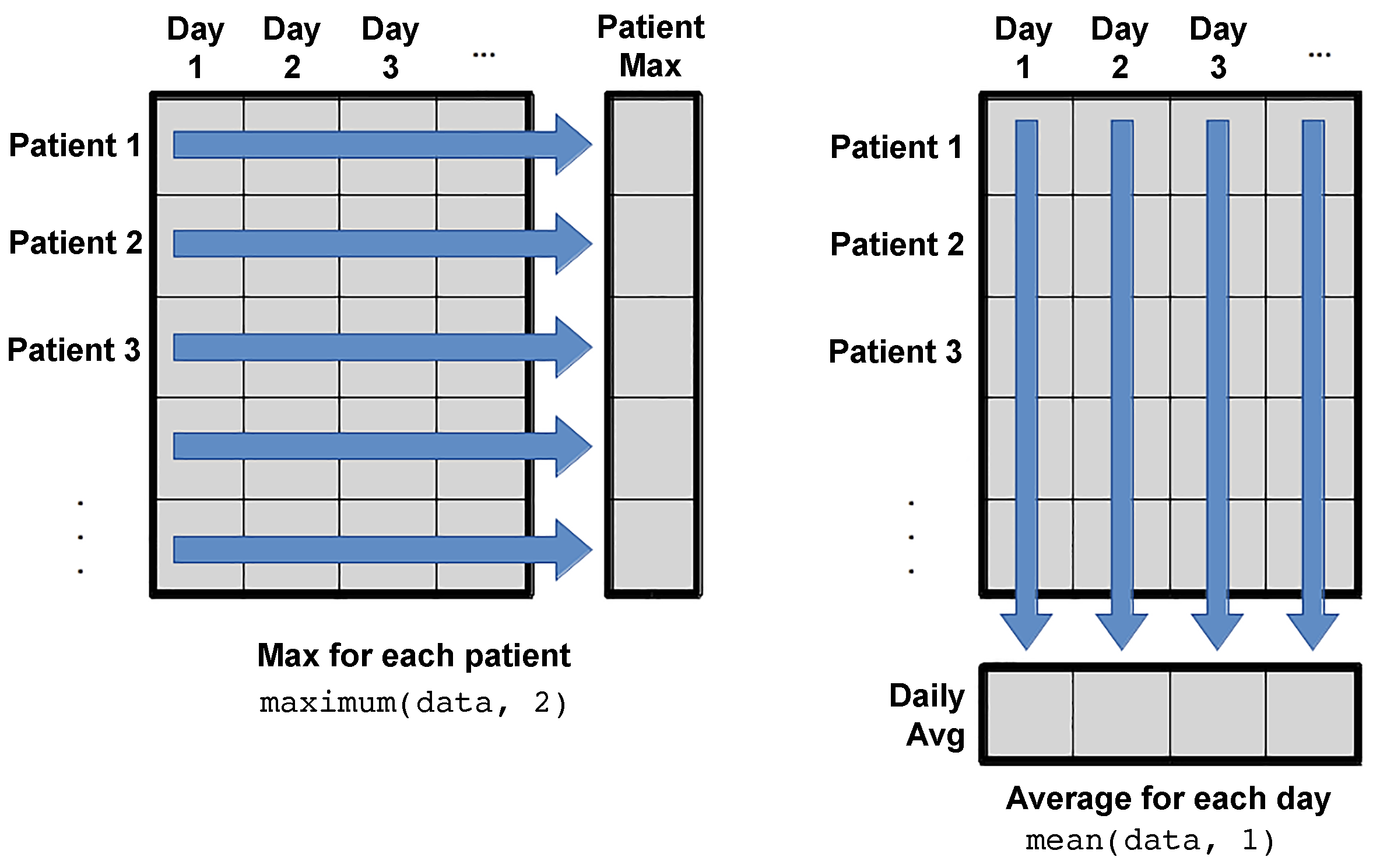
But what if you would like to do calculations for all patients (across the rows) or for all days (across the columns)? There should be an automatic way to do that kind of operations. Let’s have a look at the documentation of the maximum function.
?maximum
There is an argument in the maximum function called dims, which can be either 1 or 2 if you would like to apply the function across the columns or the rows, respectively.
Let’s check the size of the output when we use dims=1
size(maximum(data,1))
(1, 40)
or dims=2
size(mean(data,2))
(60, 1)
In the first case with dims=1, the output is an array consists of 1 row and 40 columns, which indicates that we have one value for each column (calculations across the columns or days in our case). In the case of dims=2, the size is (60,1), indicating that there are values for each row (for each patient).
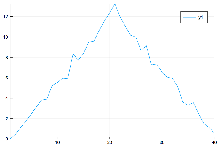
Now that we know how to perform operations across the rows and columns, let’s create a plot for the average inflammation per day. First, we calculate the average inflammation per day and we store it to a new array called avg_inflammation. Then, we transpose this array to be in the form of (1,60), i.e. 1 row and 60 columns, and not the opposite in order to pass it in the plot. We also create an array called day, which includes the number of the days. After that, we are ready to plot the average inflammation per day using the plot function:
avg_inflammation = mean(data,1);
avg_inflammation = avg_inflammation';
days=1:40;
plot(days,avg_inflammation)
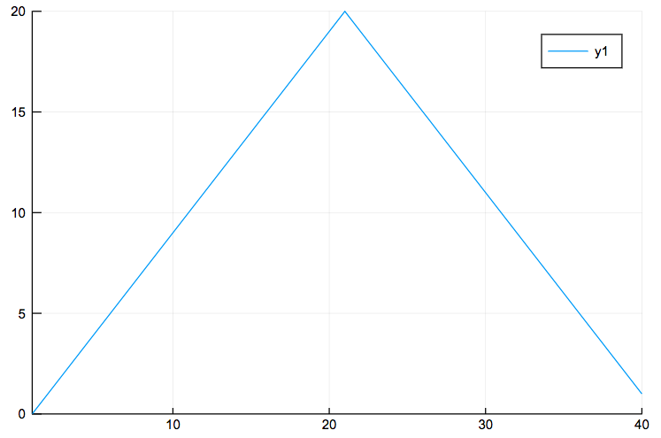
You can do the same, but now for the maximum inflammation per day:
plot(days,maximum(data,1)')
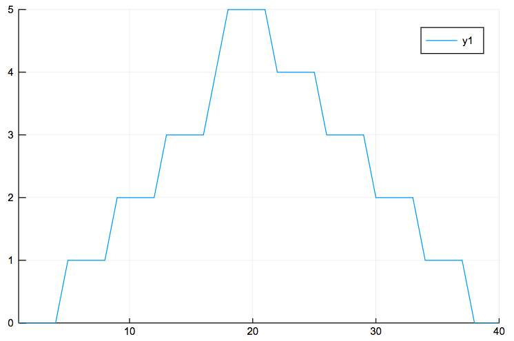
and the minimum inflammation per day:
plot(days,minimum(data,1)')
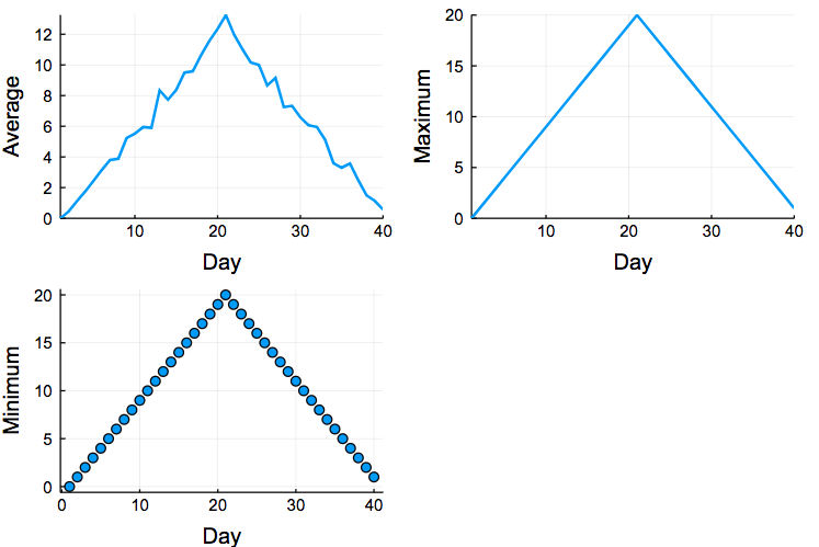
Now, it would be nice to have these three figures together. You can do that by plotting them as subfigures:
data = readdlm("./data/inflammation-01.csv", ',');

plot(plot(days,mean(data,1)', ylabel="Average", label="Mean"),
     plot(days,maximum(data,1)', ylabel="Maximum", label="Max"),
     plot(days,maximum(data,1)',
        seriestype=:scatter, ylabel="Minimum", label="Min"), lw=2, xlabel="Day", legend=false, size=(600,400)
)
where we also define the labels for the x and y axis and also the title of each subfigure.
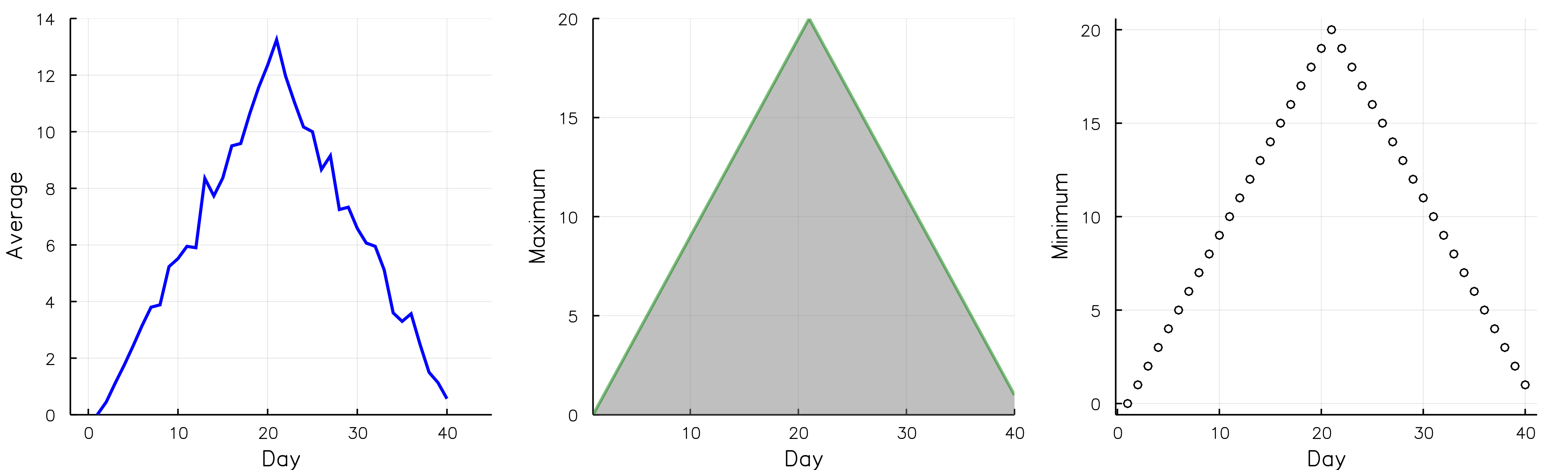
If you would like to modify the aesthetics of the plots, here is an example, where we modify the color of the line, the type of the plot, the x and y axis limits etc.
data = readdlm("./data/inflammation-01.csv", ',');

p1=plot(days,mean(data,1)', ylabel="Average", label="Mean", color="blue", xlims=(-2,45), ylims=(0,14))
p2=plot(days,maximum(data,1)', ylabel="Maximum", label="Max", c="green",alpha=0.5, fill=(0,"gray"))
#marker="white", markersize=5, markershape=:s) #:o, :x
p3=plot(days,maximum(data,1)', seriestype=:scatter, ylabel="Minimum", label="Min", marker=(:white,2,:o,stroke(1,:black))) #:o, :x

plot(p1,p2,p3,layout=(1,3), legend=false, xlabel="Day", lw=2, size=(1000,300), grid=true)
If you would like to export the plot, you need to pass the final plot into a variable and then use the savefig command to export it:
pfinal=plot(p1,p2,p3,layout=(1,3), legend=false, xlabel="Day", lw=2, size=(1000,300), grid=true)
savefig(pfinal,"myplot.png")
In this example, we pass the plot into a variable called pfinal and we use the savefig function to save the plot as “myplot.png” in my current directory (where this script is).
However, if you pass the plot into a variable, Jupyter does not display the plot anymore. If you would like to display the plot, you need to use the display function:
display(pfinal)