Learning objectives:
- …
- …
- …
At this point, we have written code to draw some interesting features in our inflammation data, loop over all our data files to quickly draw these plots for each of them, and have Julia make decisions based on what it sees in our data. But, our code is getting pretty long and complicated. What if we had thousands of datasets, and didn’t want to generate a figure for every single one? Commenting out the figure-drawing code is a nuisance. Also, what if we want to use that code again, on a different dataset or at a different point in our program? Cutting and pasting it is going to make our code get very long and very repetitive, very quickly. We’d like a way to package our code so that it is easier to reuse, and Julia provides this by letting us define things called ‘functions’ — a shorthand way of re-executing longer pieces of code.
Below you can see the generic syntax to create a function in Julia:
function function_name(argument1, argument2, ...)
  do things
end
Let’s start by creating a function called fahr_to_celsius that converts temperature from Fahrenheit to Celsius:
function fahr_to_celsius(temperature)
   (temperature-32)*(5/9)
end
Let’s now test our function by converting a temperature of 32 Fahrenheit to Celsius
println("Freezing point of water: ", fahr_to_celsius(32), " C")
Freezing point of water: 0.0 C
In Julia, as we learnt in loops and conditionals before, there is an alternative and more compact way to declare the function in a single line:
fahr_to_celsius2(temperature) = (temperature-32)*(5/9)
If you convert 32 Fahrenheit to Celsius using the fahr_to_celsius2 function, you will get the same answer:
println("Freezing point of water: ", fahr_to_celsius2(32), " C")
Freezing point of water: 0.0 C
You can also create a so called “anonymous” function, without giving a function name, using either of these syntaxes:
??????temperature -> (temperature-32)*(5/9)

function (temperature)
    (temperature-32)*(5/9)
end
?????????????
This creates a function taking one argument temperature and returning the value of the (temperature-32)(5/9)* at that value. Notice that the result is a generic function, but with a compiler-generated name based on consecutive numbering. The primary use for anonymous functions is passing them to functions which take other functions as arguments. A classic example is the map() function, which applies a function to each value of an array and returns a new array containing the resulting values. We will talk about the map() function later in this section.
Let’s create now a function that converts Celsius to Kelvin.
function celsius_to_kelvin(temperature_c)
    temperature_c += 273.15
end
and let’s test the function to convert a temperature from Celsius to Kelvin:
celsius_to_kelvin(0)
273.15
So now, if you would like to create a function to convert Fahrenheit to Kelvin, you can do it using the two functions you previously created, namely fahr_to_celsius and celsius_to_kelvin:
function fahr_to_kelvin(temperature_f)
    temperature_c = fahr_to_celsius(temperature_f)
    temperature_k = celsius_to_kelvin(temperature_c)
end
Now, if you test the function for a temperature of 212 Fahrenheit, you will get a temperature of 373.15 Kelvin. Note that the ouput value will correspond to the temperature_k variable within the function as it is the last calculated variable within the function. Of course, you can always return more outputs from your function, which we will learn how to do it in the next subsection.
fahr_to_kelvin(212)
373.15
It is good to know that there is an alternative way to do the previous convertion, i.e. you could have chained the two functions in order to get the same result without creating another function:
celsius_to_kelvin(fahr_to_celsius(212))
373.15
In this case, first we convert the temperature of 212 Fahrenheit to Celsius, and then we pass this new value (in Celsius) as an input in the celsius_to_kelvin function, with the final result being in Kelvin.
By default, the function will return the value of the last variable that was defined within the function. For example, the fahr_to_kelvin function will return the value of the temperature_k variable, which is the last command within the function. If we would like to return more than one values, we need to add a command called return before the end of the function. For example:
function fahr_to_kelvin(temperature_f)
    temperature_c = fahr_to_celsius(temperature_f)
    temperature_k = celcius_to_kelvin(temperature_c)
    return temperature_c, temperature_k
end

a, b = fahr_to_kelvin(10)
(-12.222222222222223, 260.92777777777775)
In Julia, another way to return multiple values without using the return command is:
function new_function(a,b)
    a+b, a-b
end

x, y = new_function(1,3)
(4, -2)
Although most of the functions have many arguments, you usually call them using only a few. This means that the other arguments of the function have default values. To define arguments with default values in the function, you have to use the assign (=) symbol when you define them:
function myprint(a,b=1,c=10)
    println("a:",a," b:",b," c:",c)
end

myprint(1)
In this example, the arguments b and c have a default value of 1 and 10, respectively. This way, when we call the function without defining the b and c arguments, the function will run and the arguments b and c will take their default values.
a:1 b:1 c:10
If I would like to overwrite the default values then:
myprint(1,5)
a:1 b:5 c:10
?????????????????Be careful! The order you define the arguments when you call the function is important. In the example of myprint(1,5), 1 will be assigned to the argument a, 5 will replace the default value of argument b, and since we haven’t defined a value for the argument c, it will have its default value, i.e. 10. However, if, when you call the function, you define the name of the argument, then the order is not important. For example, the order is important in this case, if we would like to define a=1 and b=5
myprint(1,5)
however the order is not important in the following example
myprint(b=5,a=1)
Multiple dispatch makes software generic and fast! Let’s start by exploring an example. We can declare functions in Julia without giving Julia any information about the types of the input arguments that function will receive:
f(x) = (2*x)^3
and then Julia will determine on its own which input argument types make sense and which do not:
f(10)
??????????????????
or
f([1, 2, 3])
??????????????????
However, we also have the option to tell Julia explicitly what types our input arguments are allowed to have. For example, let’s write a function called my_func that only takes strings as inputs.
my_funct(a::String, b::String) = println("My inputs a and b are both strings!")
You can see here that in order to restrict the type of x and y to Strings, we just follow the input argument name by a double colon (::) and the keyword String, which indicates the accepted type.
Now we’ll see if the my_func function works on Strings
my_funct("hello", "hi!")
and doesn’t work on other input argument types.
my_func(3, 4)
Now my_func works on integers! But, my_func also still works when x and y are strings!
my_func("hello", "hi!")
This is starting to get to the heart of multiple dispatch. When we declared
my_func(a::Int, b::Int) = println(“My inputs a and b are both integers!”)
we didn’t overwrite or replace
my_func(a::String, b::String)
Instead, we just added an additional method to the generic function called my_func. A generic function is the abstract concept associated with a particular operation. For example, the generic function + represents the concept of addition. A method is a specific implementation of a generic function for particular argument types. For example, + has methods that accept floating point numbers, integers, matrices, etc. We can use the methods command to see how many methods there are for my_func.
methods(my_func)
So, we now can call my_func on integers or strings. When you call my_func on a particular set of arguments, Julia will infer the types of the inputs and dispatch the appropriate method. This is the concept behind the multiple dispatch.
Multiple dispatch makes our code generic and fast. Our code can be generic and flexible because we can write code in terms of abstract operations such as addition and multiplication, rather than in terms of specific implementations. At the same time, our code runs quickly because Julia is able to call efficient methods for the relevant types.
To see which method is being dispatched when you call a generic function, you can use the @which macro:
@which my_func(3, 4)
And we can continue to add other methods to our generic function foo. Let’s add one that takes the abstract type Number, which includes subtypes such as Int, Float64, and other objects you would think of as numbers:
my_func(a::Number, b::Number) = println("My inputs a and b are both numbers!")
We can also add a fallback, duck-typed method for foo that takes inputs of any type:
my_func(a, b) = println("I accept inputs of any type!")
##Exercise
By convention, functions followed by the exclamation mark symbol (!) can mutate its inputs. Any function can mutate its inputs, but so that it is clear that it is doing so, we suffix it with a !
For example let’s use the sort function to sort a list of values
v = [3,5,2]
sort(v)
3-element Array{Int64,1}:
 2
 3
 5
However, list v hasn’t changed
v
3-element Array{Int64,1}:
 3
 5
 2
Now if we run the sort function but with the !, the list will retain the sorted format because we used the ! after the sort function:
sort!(v)
3-element Array{Int64,1}:
 2
 3
 5
v
3-element Array{Int64,1}:
 2
 3
 5
The map function is a “higher-order” function in Julia that takes a function as one of its input arguments. map then applies that function to every element of the data structure you pass it. For example, executing
map(f, [1, 2, 3])
will give you an output array where the function f has been applied to all elements of [1,2,3], i.e. [f(1),f(2),f(3)].
Here is an example. We have a function that calculates the cube of a number and we would like to apply this calculation to a list of numbers. We are going to use the map function to do that:
map(x->x^3, [1,4,7])
3-element Array{Int64,1}:
   1
  64
 343
The broadcast function is another “higher-order” function like map. broadcast is a generilisation of map, so it can do every thing map can do and more. The syntax for calling broadcast is the same as for calling map
broadcast(function_name, [item1, item2, item3])
Some syntactic sugar for calling broadcast is to place a dot (.) between the name of the function you want to broadcast and its input arguments. For example
broadcast(function_name, [item1, item2, item3])
is the same as
function_name.([item1, item2, item3])
Let’s do an example to better understand the broadcast function.
broadcast(x->x^3, [1,4,7])
3-element Array{Int64,1}:
   1
  64
 343
We can do the same now using the dot after calling the function
f(x) = x^3
f.([1,4,7])
3-element Array{Int64,1}:
   1
  64
 343
Another example. Let’s create a 3x3 array using the compact way for nested loops in Julia
A = [i + 3*j for j in 0:2, i in 1:3]
3×3 Array{Int64,2}:
 1  2  3
 4  5  6
 7  8  9
If we run the f function on the A array,
f(A)
3×3 Array{Int64,2}:
  468   576   684
 1062  1305  1548
 1656  2034  2412
we will have the cube of all the numbers of the A array.
Now let’s try to apply the broadcast function on f using the dot syntax. This syntax for broadcasting allows us to write relatively complex compound elementwise expressions in a way that looks natural/closer to mathematical notation.
f.(A)
3×3 Array{Int64,2}:
   1    8   27
  64  125  216
 343  512  729
or a more complex example
A .+ 2 .* f.(A) ./ A
3×3 Array{Float64,2}:
   3.0   10.0   21.0
  36.0   55.0   78.0
 105.0  136.0  171.0
The function documentation syntax is very simple: any string appearing at the top-level right before an object (function, macro, type or instance) will be interpreted as documentation (these are called docstrings). Here is an example:
"This is a sample of a function documentation"
function my_func(a,b)
   println("a is:",a," while b is:",b)
end
Let’s check the documentation of my_func using the question mark
?my_func
search:

This is a sample of a function documentation
Documentation is interpreted as Markdown, so you can use indentation and code fences to delimit code examples from text. Technically, any object can be associated with any other as metadata. Markdown happens to be the default, but one can construct other string macros and pass them to the @doc macro as well.
Here is a more complex example, still using Markdown:
"""
This is a more complex function documentation:

    my_func(a,b)

- This function **prints** the arguments a and b.
- It doesn't use any default values.
"""
function my_func(a,b)
   println("a is:",a," while b is:",b)
end
check the documentation of my_func
?my_func
Please find more tips for writing documentation in this link: https://docs.julialang.org/en/stable/manual/documentation/#Documentation-1
In programming, it is really important to use names for variables and functions that are descriptive and meaningful. Otherwise, if you check your scripts after a few months, or if you share your scripts with your colleagues, it will be hard to read them and you or your colleagues will need to spend hours understanding what you are doing in the scripts. Here is an example of a non-readable function. Please spend one minute reading this function and try to understand what the function does:
function s(p)
    a=0

    for v in p
        a+=v
    end

    m=a/length(p)
    d=0

    for v in p
        d+=(v-m)*(v-m)
    end

    return sqrt(d/(length(p)-1))
end
For those who couldn’t understand what the previous functions does, please have a look in the same function but now using more descriptive and meaningful names:
function std_dev(sample)
    sample_sum=0

    for value in sample
        sample_sum+=value
    end

    sample_mean=sample_sum/length(sample)
    sum_squared_devs=0

    for value in sample
        sum_squared_devs+=(value-sample_mean)*(value-sample_mean)
    end

    return sqrt(sum_squared_devs/(length(sample)-1))
end
Is it easier to read the first or the second function?
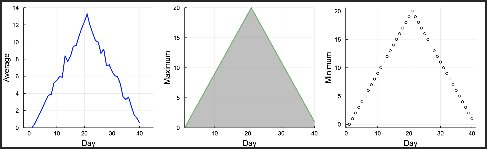
In the previous modules, we learnt how to run the analysis for multiple datasets and how to use conditionals to detect problems in our datasets. Now let’s go one step further and implement some functions to our scipt. We are going to create a function called analyze, which takes the filename as an input argument and produces the plot with the three subfigures for the average, maximum and minimum inflammation per day. Then we will create another function called detect_problems to detect if there are any problems in the inflammation dataset, which also takes the filename as an input argument.
Let’s define the analyze function first:
function analyze(filename)

    println("Processing dataset: ",filename)

    sleep(0.5)

    data = readdlm(filename, ',');
    days=1:40;

    p1=plot(days,mean(data,1)', ylabel="Average", label="Mean", color="blue", xlims=(-2,45), ylims=(0,14))
    p2=plot(days,maximum(data,1)', ylabel="Maximum", label="Max", c="green",alpha=0.5, fill=(0,"gray"))
    p3=plot(days,maximum(data,1)', seriestype=:scatter, ylabel="Minimum", label="Min", marker=(:white,2,:o,stroke(1,:black)))

    p=plot(p1,p2,p3,layout=(1,3), legend=false, xlabel="Day", lw=2,size=(1000,300), grid=true)
    display(p)

end
analyze (generic function with 1 method)
Now declare the detect_problems function, which will be:
function detect_problems(filename)

    data = readdlm(filename, ',');

    if (maximum(data,1)'[1]==0) & (maximum(data,1)'[21]==20)
        println("Suspicious looking maximum!")
    elseif sum(minimum(data,1)')==0
        println("Minimum add up to zero!")
    else
        println("The dataset is OK")
    end

end
detect_problems (generic function with 1 method)
Let’s check if the functions are working correctly using the first inflammation dataset:
analyze("./data/inflammation-01.csv")
And let’s check the detect_problems function for the third dataset as well
detect_problems("./data/inflammation-03.csv")
Minimum add up to zero!
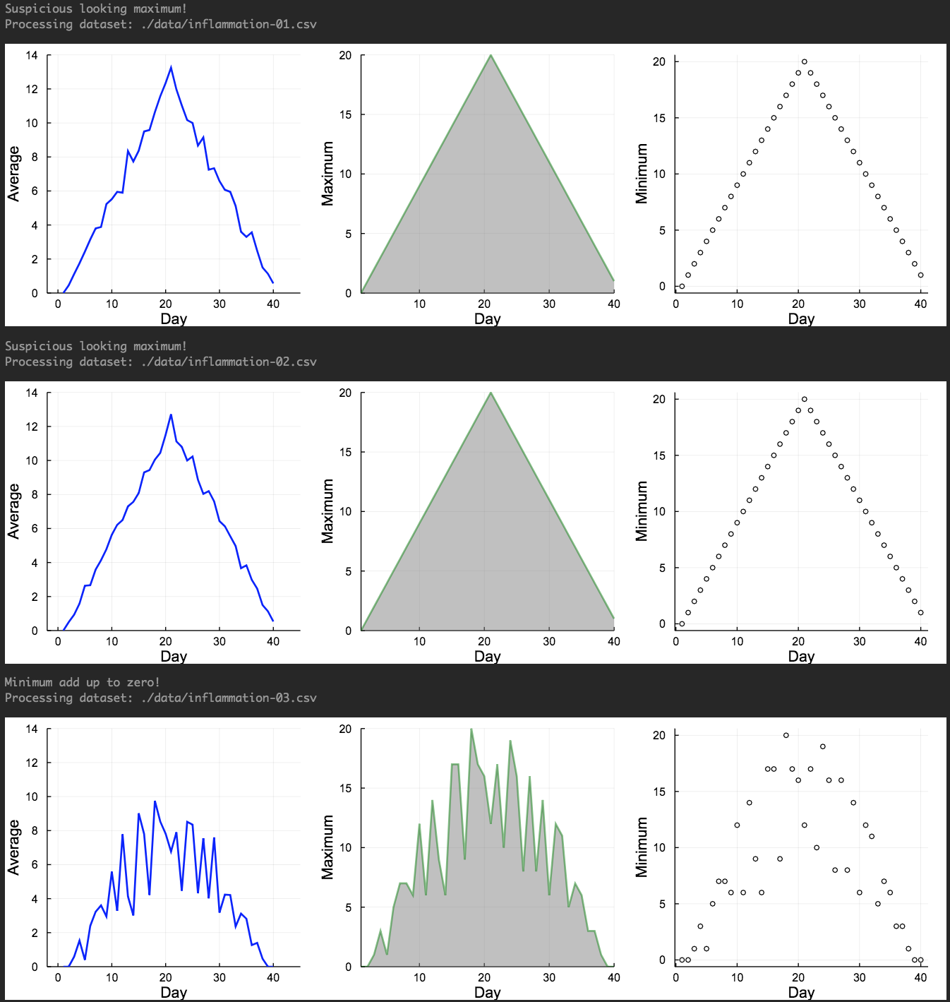
So both functions seem to work correctly. Now, we will try to combine everything we learnt until now to analyse the first three inflammation dataset using the concepts of loops, conditionals and functions:
using Plots
using Glob

filenames = sort(glob("infl*","./data/"), rev=false)

for f in filenames[1:3]
    detect_problems(f)
    analyze(f)
end